房价预测

比赛说明
- 房价预测
- 要求购房者描述他们的梦想之家,他们可能不会从地下室天花板的高度或与东西方铁路的接近度开始。但是这个游乐场比赛的数据集证明,对价格谈判的影响远远超过卧室或白色栅栏的数量。
- 有79个解释变量描述(几乎)爱荷华州埃姆斯的住宅房屋的每个方面,这个竞赛挑战你预测每个房屋的最终价格。
参赛成员
- 开源组织: ApacheCN ~ apachecn.org
比赛分析
- 回归问题:价格的问题
- 常用算法:
回归、树回归、GBDT、xgboost、lightGBM
步骤:
一. 数据分析
1. 下载并加载数据
2. 总体预览:了解每列数据的含义,数据的格式等
3. 数据初步分析,使用统计学与绘图:初步了解数据之间的相关性,为构造特征工程以及模型建立做准备

二. 特征工程
1.根据业务,常识,以及第二步的数据分析构造特征工程.
2.将特征转换为模型可以辨别的类型(如处理缺失值,处理文本进行等)

三. 模型选择
1.根据目标函数确定学习类型,是无监督学习还是监督学习,是分类问题还是回归问题等.
2.比较各个模型的分数,然后取效果较好的模型作为基础模型.

四. 模型融合
1. 可以参考泰坦尼克号的简单模型融合方式,通过对模型的对比打分方式选择合适的模型
2. 在房价预测里我们使用模型融合的方法来输出结果,最终的效果很好。

五. 修改特征和模型参数
1.可以通过添加或者修改特征,提高模型的上限.
2.通过修改模型的参数,是模型逼近上限
一. 数据分析
数据下载和加载
# 导入相关数据包
import numpy as np
import pandas as pd
import seaborn as sns
import matplotlib.pyplot as plt
%matplotlib inline

from scipy import stats
from scipy.stats import norm
root_path = '/opt/data/kaggle/getting-started/house-prices'

train = pd.read_csv('%s/%s' % (root_path, 'train.csv'))
test = pd.read_csv('%s/%s' % (root_path, 'test.csv'))
特征说明
train.columns
Index(['Id', 'MSSubClass', 'MSZoning', 'LotFrontage', 'LotArea', 'Street',
       'Alley', 'LotShape', 'LandContour', 'Utilities', 'LotConfig',
       'LandSlope', 'Neighborhood', 'Condition1', 'Condition2', 'BldgType',
       'HouseStyle', 'OverallQual', 'OverallCond', 'YearBuilt', 'YearRemodAdd',
       'RoofStyle', 'RoofMatl', 'Exterior1st', 'Exterior2nd', 'MasVnrType',
       'MasVnrArea', 'ExterQual', 'ExterCond', 'Foundation', 'BsmtQual',
       'BsmtCond', 'BsmtExposure', 'BsmtFinType1', 'BsmtFinSF1',
       'BsmtFinType2', 'BsmtFinSF2', 'BsmtUnfSF', 'TotalBsmtSF', 'Heating',
       'HeatingQC', 'CentralAir', 'Electrical', '1stFlrSF', '2ndFlrSF',
       'LowQualFinSF', 'GrLivArea', 'BsmtFullBath', 'BsmtHalfBath', 'FullBath',
       'HalfBath', 'BedroomAbvGr', 'KitchenAbvGr', 'KitchenQual',
       'TotRmsAbvGrd', 'Functional', 'Fireplaces', 'FireplaceQu', 'GarageType',
       'GarageYrBlt', 'GarageFinish', 'GarageCars', 'GarageArea', 'GarageQual',
       'GarageCond', 'PavedDrive', 'WoodDeckSF', 'OpenPorchSF',
       'EnclosedPorch', '3SsnPorch', 'ScreenPorch', 'PoolArea', 'PoolQC',
       'Fence', 'MiscFeature', 'MiscVal', 'MoSold', 'YrSold', 'SaleType',
       'SaleCondition', 'SalePrice'],
      dtype='object')
train.info()
<class 'pandas.core.frame.DataFrame'>
RangeIndex: 1460 entries, 0 to 1459
Data columns (total 81 columns):
Id               1460 non-null int64
MSSubClass       1460 non-null int64
MSZoning         1460 non-null object
LotFrontage      1201 non-null float64
LotArea          1460 non-null int64
Street           1460 non-null object
Alley            91 non-null object
LotShape         1460 non-null object
LandContour      1460 non-null object
Utilities        1460 non-null object
LotConfig        1460 non-null object
LandSlope        1460 non-null object
Neighborhood     1460 non-null object
Condition1       1460 non-null object
Condition2       1460 non-null object
BldgType         1460 non-null object
HouseStyle       1460 non-null object
OverallQual      1460 non-null int64
OverallCond      1460 non-null int64
YearBuilt        1460 non-null int64
YearRemodAdd     1460 non-null int64
RoofStyle        1460 non-null object
RoofMatl         1460 non-null object
Exterior1st      1460 non-null object
Exterior2nd      1460 non-null object
MasVnrType       1452 non-null object
MasVnrArea       1452 non-null float64
ExterQual        1460 non-null object
ExterCond        1460 non-null object
Foundation       1460 non-null object
BsmtQual         1423 non-null object
BsmtCond         1423 non-null object
BsmtExposure     1422 non-null object
BsmtFinType1     1423 non-null object
BsmtFinSF1       1460 non-null int64
BsmtFinType2     1422 non-null object
BsmtFinSF2       1460 non-null int64
BsmtUnfSF        1460 non-null int64
TotalBsmtSF      1460 non-null int64
Heating          1460 non-null object
HeatingQC        1460 non-null object
CentralAir       1460 non-null object
Electrical       1459 non-null object
1stFlrSF         1460 non-null int64
2ndFlrSF         1460 non-null int64
LowQualFinSF     1460 non-null int64
GrLivArea        1460 non-null int64
BsmtFullBath     1460 non-null int64
BsmtHalfBath     1460 non-null int64
FullBath         1460 non-null int64
HalfBath         1460 non-null int64
BedroomAbvGr     1460 non-null int64
KitchenAbvGr     1460 non-null int64
KitchenQual      1460 non-null object
TotRmsAbvGrd     1460 non-null int64
Functional       1460 non-null object
Fireplaces       1460 non-null int64
FireplaceQu      770 non-null object
GarageType       1379 non-null object
GarageYrBlt      1379 non-null float64
GarageFinish     1379 non-null object
GarageCars       1460 non-null int64
GarageArea       1460 non-null int64
GarageQual       1379 non-null object
GarageCond       1379 non-null object
PavedDrive       1460 non-null object
WoodDeckSF       1460 non-null int64
OpenPorchSF      1460 non-null int64
EnclosedPorch    1460 non-null int64
3SsnPorch        1460 non-null int64
ScreenPorch      1460 non-null int64
PoolArea         1460 non-null int64
PoolQC           7 non-null object
Fence            281 non-null object
MiscFeature      54 non-null object
MiscVal          1460 non-null int64
MoSold           1460 non-null int64
YrSold           1460 non-null int64
SaleType         1460 non-null object
SaleCondition    1460 non-null object
SalePrice        1460 non-null int64
dtypes: float64(3), int64(35), object(43)
memory usage: 924.0+ KB
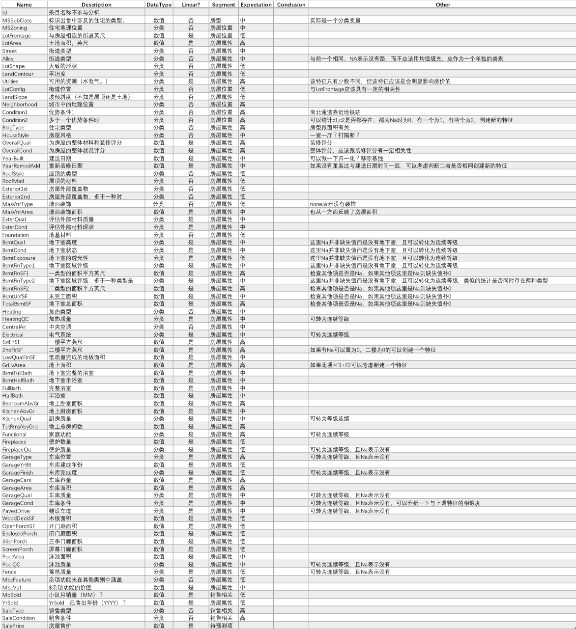
特征详情
train.head(5)
| Id | MSSubClass | MSZoning | LotFrontage | LotArea | Street | Alley | LotShape | LandContour | Utilities | ... | PoolArea | PoolQC | Fence | MiscFeature | MiscVal | MoSold | YrSold | SaleType | SaleCondition | SalePrice | |
|---|---|---|---|---|---|---|---|---|---|---|---|---|---|---|---|---|---|---|---|---|---|
| 0 | 1 | 60 | RL | 65.0 | 8450 | Pave | NaN | Reg | Lvl | AllPub | ... | 0 | NaN | NaN | NaN | 0 | 2 | 2008 | WD | Normal | 208500 |
| 1 | 2 | 20 | RL | 80.0 | 9600 | Pave | NaN | Reg | Lvl | AllPub | ... | 0 | NaN | NaN | NaN | 0 | 5 | 2007 | WD | Normal | 181500 |
| 2 | 3 | 60 | RL | 68.0 | 11250 | Pave | NaN | IR1 | Lvl | AllPub | ... | 0 | NaN | NaN | NaN | 0 | 9 | 2008 | WD | Normal | 223500 |
| 3 | 4 | 70 | RL | 60.0 | 9550 | Pave | NaN | IR1 | Lvl | AllPub | ... | 0 | NaN | NaN | NaN | 0 | 2 | 2006 | WD | Abnorml | 140000 |
| 4 | 5 | 60 | RL | 84.0 | 14260 | Pave | NaN | IR1 | Lvl | AllPub | ... | 0 | NaN | NaN | NaN | 0 | 12 | 2008 | WD | Normal | 250000 |
5 rows × 81 columns
特征分析(统计学与绘图)
每一行是一条房子出售的记录,原始特征有80列,具体的意思可以根据data_description来查询,我们要预测的是房子的售价,即“SalePrice”。训练集有1459条记录,测试集有1460条记录,数据量还是很小的。
# 相关性协方差表,corr()函数,返回结果接近0说明无相关性,大于0说明是正相关,小于0是负相关.
train_corr = train.drop('Id',axis=1).corr()
train_corr
| MSSubClass | LotFrontage | LotArea | OverallQual | OverallCond | YearBuilt | YearRemodAdd | MasVnrArea | BsmtFinSF1 | BsmtFinSF2 | ... | WoodDeckSF | OpenPorchSF | EnclosedPorch | 3SsnPorch | ScreenPorch | PoolArea | MiscVal | MoSold | YrSold | SalePrice | |
|---|---|---|---|---|---|---|---|---|---|---|---|---|---|---|---|---|---|---|---|---|---|
| MSSubClass | 1.000000 | -0.386347 | -0.139781 | 0.032628 | -0.059316 | 0.027850 | 0.040581 | 0.022936 | -0.069836 | -0.065649 | ... | -0.012579 | -0.006100 | -0.012037 | -0.043825 | -0.026030 | 0.008283 | -0.007683 | -0.013585 | -0.021407 | -0.084284 |
| LotFrontage | -0.386347 | 1.000000 | 0.426095 | 0.251646 | -0.059213 | 0.123349 | 0.088866 | 0.193458 | 0.233633 | 0.049900 | ... | 0.088521 | 0.151972 | 0.010700 | 0.070029 | 0.041383 | 0.206167 | 0.003368 | 0.011200 | 0.007450 | 0.351799 |
| LotArea | -0.139781 | 0.426095 | 1.000000 | 0.105806 | -0.005636 | 0.014228 | 0.013788 | 0.104160 | 0.214103 | 0.111170 | ... | 0.171698 | 0.084774 | -0.018340 | 0.020423 | 0.043160 | 0.077672 | 0.038068 | 0.001205 | -0.014261 | 0.263843 |
| OverallQual | 0.032628 | 0.251646 | 0.105806 | 1.000000 | -0.091932 | 0.572323 | 0.550684 | 0.411876 | 0.239666 | -0.059119 | ... | 0.238923 | 0.308819 | -0.113937 | 0.030371 | 0.064886 | 0.065166 | -0.031406 | 0.070815 | -0.027347 | 0.790982 |
| OverallCond | -0.059316 | -0.059213 | -0.005636 | -0.091932 | 1.000000 | -0.375983 | 0.073741 | -0.128101 | -0.046231 | 0.040229 | ... | -0.003334 | -0.032589 | 0.070356 | 0.025504 | 0.054811 | -0.001985 | 0.068777 | -0.003511 | 0.043950 | -0.077856 |
| YearBuilt | 0.027850 | 0.123349 | 0.014228 | 0.572323 | -0.375983 | 1.000000 | 0.592855 | 0.315707 | 0.249503 | -0.049107 | ... | 0.224880 | 0.188686 | -0.387268 | 0.031355 | -0.050364 | 0.004950 | -0.034383 | 0.012398 | -0.013618 | 0.522897 |
| YearRemodAdd | 0.040581 | 0.088866 | 0.013788 | 0.550684 | 0.073741 | 0.592855 | 1.000000 | 0.179618 | 0.128451 | -0.067759 | ... | 0.205726 | 0.226298 | -0.193919 | 0.045286 | -0.038740 | 0.005829 | -0.010286 | 0.021490 | 0.035743 | 0.507101 |
| MasVnrArea | 0.022936 | 0.193458 | 0.104160 | 0.411876 | -0.128101 | 0.315707 | 0.179618 | 1.000000 | 0.264736 | -0.072319 | ... | 0.159718 | 0.125703 | -0.110204 | 0.018796 | 0.061466 | 0.011723 | -0.029815 | -0.005965 | -0.008201 | 0.477493 |
| BsmtFinSF1 | -0.069836 | 0.233633 | 0.214103 | 0.239666 | -0.046231 | 0.249503 | 0.128451 | 0.264736 | 1.000000 | -0.050117 | ... | 0.204306 | 0.111761 | -0.102303 | 0.026451 | 0.062021 | 0.140491 | 0.003571 | -0.015727 | 0.014359 | 0.386420 |
| BsmtFinSF2 | -0.065649 | 0.049900 | 0.111170 | -0.059119 | 0.040229 | -0.049107 | -0.067759 | -0.072319 | -0.050117 | 1.000000 | ... | 0.067898 | 0.003093 | 0.036543 | -0.029993 | 0.088871 | 0.041709 | 0.004940 | -0.015211 | 0.031706 | -0.011378 |
| BsmtUnfSF | -0.140759 | 0.132644 | -0.002618 | 0.308159 | -0.136841 | 0.149040 | 0.181133 | 0.114442 | -0.495251 | -0.209294 | ... | -0.005316 | 0.129005 | -0.002538 | 0.020764 | -0.012579 | -0.035092 | -0.023837 | 0.034888 | -0.041258 | 0.214479 |
| TotalBsmtSF | -0.238518 | 0.392075 | 0.260833 | 0.537808 | -0.171098 | 0.391452 | 0.291066 | 0.363936 | 0.522396 | 0.104810 | ... | 0.232019 | 0.247264 | -0.095478 | 0.037384 | 0.084489 | 0.126053 | -0.018479 | 0.013196 | -0.014969 | 0.613581 |
| 1stFlrSF | -0.251758 | 0.457181 | 0.299475 | 0.476224 | -0.144203 | 0.281986 | 0.240379 | 0.344501 | 0.445863 | 0.097117 | ... | 0.235459 | 0.211671 | -0.065292 | 0.056104 | 0.088758 | 0.131525 | -0.021096 | 0.031372 | -0.013604 | 0.605852 |
| 2ndFlrSF | 0.307886 | 0.080177 | 0.050986 | 0.295493 | 0.028942 | 0.010308 | 0.140024 | 0.174561 | -0.137079 | -0.099260 | ... | 0.092165 | 0.208026 | 0.061989 | -0.024358 | 0.040606 | 0.081487 | 0.016197 | 0.035164 | -0.028700 | 0.319334 |
| LowQualFinSF | 0.046474 | 0.038469 | 0.004779 | -0.030429 | 0.025494 | -0.183784 | -0.062419 | -0.069071 | -0.064503 | 0.014807 | ... | -0.025444 | 0.018251 | 0.061081 | -0.004296 | 0.026799 | 0.062157 | -0.003793 | -0.022174 | -0.028921 | -0.025606 |
| GrLivArea | 0.074853 | 0.402797 | 0.263116 | 0.593007 | -0.079686 | 0.199010 | 0.287389 | 0.390857 | 0.208171 | -0.009640 | ... | 0.247433 | 0.330224 | 0.009113 | 0.020643 | 0.101510 | 0.170205 | -0.002416 | 0.050240 | -0.036526 | 0.708624 |
| BsmtFullBath | 0.003491 | 0.100949 | 0.158155 | 0.111098 | -0.054942 | 0.187599 | 0.119470 | 0.085310 | 0.649212 | 0.158678 | ... | 0.175315 | 0.067341 | -0.049911 | -0.000106 | 0.023148 | 0.067616 | -0.023047 | -0.025361 | 0.067049 | 0.227122 |
| BsmtHalfBath | -0.002333 | -0.007234 | 0.048046 | -0.040150 | 0.117821 | -0.038162 | -0.012337 | 0.026673 | 0.067418 | 0.070948 | ... | 0.040161 | -0.025324 | -0.008555 | 0.035114 | 0.032121 | 0.020025 | -0.007367 | 0.032873 | -0.046524 | -0.016844 |
| FullBath | 0.131608 | 0.198769 | 0.126031 | 0.550600 | -0.194149 | 0.468271 | 0.439046 | 0.276833 | 0.058543 | -0.076444 | ... | 0.187703 | 0.259977 | -0.115093 | 0.035353 | -0.008106 | 0.049604 | -0.014290 | 0.055872 | -0.019669 | 0.560664 |
| HalfBath | 0.177354 | 0.053532 | 0.014259 | 0.273458 | -0.060769 | 0.242656 | 0.183331 | 0.201444 | 0.004262 | -0.032148 | ... | 0.108080 | 0.199740 | -0.095317 | -0.004972 | 0.072426 | 0.022381 | 0.001290 | -0.009050 | -0.010269 | 0.284108 |
| BedroomAbvGr | -0.023438 | 0.263170 | 0.119690 | 0.101676 | 0.012980 | -0.070651 | -0.040581 | 0.102821 | -0.107355 | -0.015728 | ... | 0.046854 | 0.093810 | 0.041570 | -0.024478 | 0.044300 | 0.070703 | 0.007767 | 0.046544 | -0.036014 | 0.168213 |
| KitchenAbvGr | 0.281721 | -0.006069 | -0.017784 | -0.183882 | -0.087001 | -0.174800 | -0.149598 | -0.037610 | -0.081007 | -0.040751 | ... | -0.090130 | -0.070091 | 0.037312 | -0.024600 | -0.051613 | -0.014525 | 0.062341 | 0.026589 | 0.031687 | -0.135907 |
| TotRmsAbvGrd | 0.040380 | 0.352096 | 0.190015 | 0.427452 | -0.057583 | 0.095589 | 0.191740 | 0.280682 | 0.044316 | -0.035227 | ... | 0.165984 | 0.234192 | 0.004151 | -0.006683 | 0.059383 | 0.083757 | 0.024763 | 0.036907 | -0.034516 | 0.533723 |
| Fireplaces | -0.045569 | 0.266639 | 0.271364 | 0.396765 | -0.023820 | 0.147716 | 0.112581 | 0.249070 | 0.260011 | 0.046921 | ... | 0.200019 | 0.169405 | -0.024822 | 0.011257 | 0.184530 | 0.095074 | 0.001409 | 0.046357 | -0.024096 | 0.466929 |
| GarageYrBlt | 0.085072 | 0.070250 | -0.024947 | 0.547766 | -0.324297 | 0.825667 | 0.642277 | 0.252691 | 0.153484 | -0.088011 | ... | 0.224577 | 0.228425 | -0.297003 | 0.023544 | -0.075418 | -0.014501 | -0.032417 | 0.005337 | -0.001014 | 0.486362 |
| GarageCars | -0.040110 | 0.285691 | 0.154871 | 0.600671 | -0.185758 | 0.537850 | 0.420622 | 0.364204 | 0.224054 | -0.038264 | ... | 0.226342 | 0.213569 | -0.151434 | 0.035765 | 0.050494 | 0.020934 | -0.043080 | 0.040522 | -0.039117 | 0.640409 |
| GarageArea | -0.098672 | 0.344997 | 0.180403 | 0.562022 | -0.151521 | 0.478954 | 0.371600 | 0.373066 | 0.296970 | -0.018227 | ... | 0.224666 | 0.241435 | -0.121777 | 0.035087 | 0.051412 | 0.061047 | -0.027400 | 0.027974 | -0.027378 | 0.623431 |
| WoodDeckSF | -0.012579 | 0.088521 | 0.171698 | 0.238923 | -0.003334 | 0.224880 | 0.205726 | 0.159718 | 0.204306 | 0.067898 | ... | 1.000000 | 0.058661 | -0.125989 | -0.032771 | -0.074181 | 0.073378 | -0.009551 | 0.021011 | 0.022270 | 0.324413 |
| OpenPorchSF | -0.006100 | 0.151972 | 0.084774 | 0.308819 | -0.032589 | 0.188686 | 0.226298 | 0.125703 | 0.111761 | 0.003093 | ... | 0.058661 | 1.000000 | -0.093079 | -0.005842 | 0.074304 | 0.060762 | -0.018584 | 0.071255 | -0.057619 | 0.315856 |
| EnclosedPorch | -0.012037 | 0.010700 | -0.018340 | -0.113937 | 0.070356 | -0.387268 | -0.193919 | -0.110204 | -0.102303 | 0.036543 | ... | -0.125989 | -0.093079 | 1.000000 | -0.037305 | -0.082864 | 0.054203 | 0.018361 | -0.028887 | -0.009916 | -0.128578 |
| 3SsnPorch | -0.043825 | 0.070029 | 0.020423 | 0.030371 | 0.025504 | 0.031355 | 0.045286 | 0.018796 | 0.026451 | -0.029993 | ... | -0.032771 | -0.005842 | -0.037305 | 1.000000 | -0.031436 | -0.007992 | 0.000354 | 0.029474 | 0.018645 | 0.044584 |
| ScreenPorch | -0.026030 | 0.041383 | 0.043160 | 0.064886 | 0.054811 | -0.050364 | -0.038740 | 0.061466 | 0.062021 | 0.088871 | ... | -0.074181 | 0.074304 | -0.082864 | -0.031436 | 1.000000 | 0.051307 | 0.031946 | 0.023217 | 0.010694 | 0.111447 |
| PoolArea | 0.008283 | 0.206167 | 0.077672 | 0.065166 | -0.001985 | 0.004950 | 0.005829 | 0.011723 | 0.140491 | 0.041709 | ... | 0.073378 | 0.060762 | 0.054203 | -0.007992 | 0.051307 | 1.000000 | 0.029669 | -0.033737 | -0.059689 | 0.092404 |
| MiscVal | -0.007683 | 0.003368 | 0.038068 | -0.031406 | 0.068777 | -0.034383 | -0.010286 | -0.029815 | 0.003571 | 0.004940 | ... | -0.009551 | -0.018584 | 0.018361 | 0.000354 | 0.031946 | 0.029669 | 1.000000 | -0.006495 | 0.004906 | -0.021190 |
| MoSold | -0.013585 | 0.011200 | 0.001205 | 0.070815 | -0.003511 | 0.012398 | 0.021490 | -0.005965 | -0.015727 | -0.015211 | ... | 0.021011 | 0.071255 | -0.028887 | 0.029474 | 0.023217 | -0.033737 | -0.006495 | 1.000000 | -0.145721 | 0.046432 |
| YrSold | -0.021407 | 0.007450 | -0.014261 | -0.027347 | 0.043950 | -0.013618 | 0.035743 | -0.008201 | 0.014359 | 0.031706 | ... | 0.022270 | -0.057619 | -0.009916 | 0.018645 | 0.010694 | -0.059689 | 0.004906 | -0.145721 | 1.000000 | -0.028923 |
| SalePrice | -0.084284 | 0.351799 | 0.263843 | 0.790982 | -0.077856 | 0.522897 | 0.507101 | 0.477493 | 0.386420 | -0.011378 | ... | 0.324413 | 0.315856 | -0.128578 | 0.044584 | 0.111447 | 0.092404 | -0.021190 | 0.046432 | -0.028923 | 1.000000 |
37 rows × 37 columns
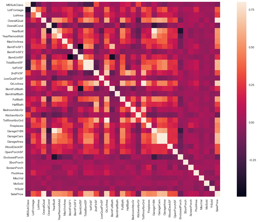
所有特征相关度分析
# 画出相关性热力图
a = plt.subplots(figsize=(20, 12))#调整画布大小
a = sns.heatmap(train_corr, vmax=.8, square=True)#画热力图   annot=True 显示系数
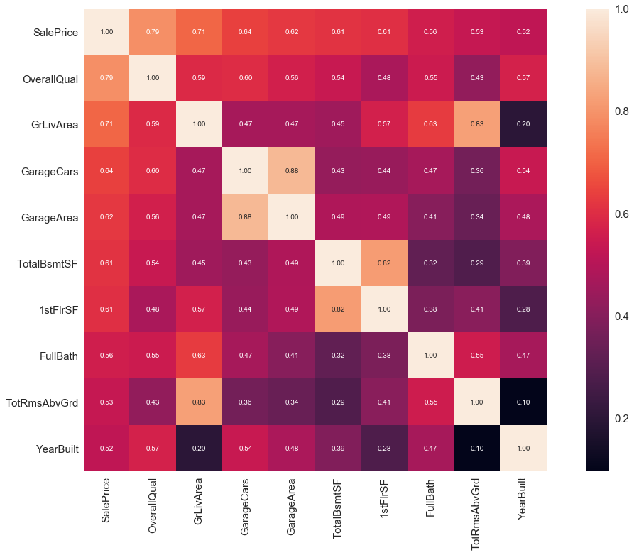
SalePrice 相关度特征排序
# 寻找K个最相关的特征信息
k = 10 # number of variables for heatmap
cols = train_corr.nlargest(k, 'SalePrice')['SalePrice'].index
cm = np.corrcoef(train[cols].values.T)
sns.set(font_scale=1.5)
hm = plt.subplots(figsize=(20, 12))#调整画布大小
hm = sns.heatmap(cm, cbar=True, annot=True, square=True, fmt='.2f', annot_kws={'size': 10}, yticklabels=cols.values, xticklabels=cols.values)
plt.show()

'''
1. GarageCars 和 GarageAre 相关性很高、就像双胞胎一样,所以我们只需要其中的一个变量,例如:GarageCars。
2. TotalBsmtSF  和 1stFloor 与上述情况相同,我们选择 TotalBsmtS
3. GarageAre 和 TotRmsAbvGrd 与上述情况相同,我们选择 GarageAre
'''
'\n1. GarageCars 和 GarageAre 相关性很高、就像双胞胎一样,所以我们只需要其中的一个变量,例如:GarageCars。\n2. TotalBsmtSF 和 1stFloor 与上述情况相同,我们选择 TotalBsmtS\n3. GarageAre 和 TotRmsAbvGrd 与上述情况相同,我们选择 GarageAre\n'
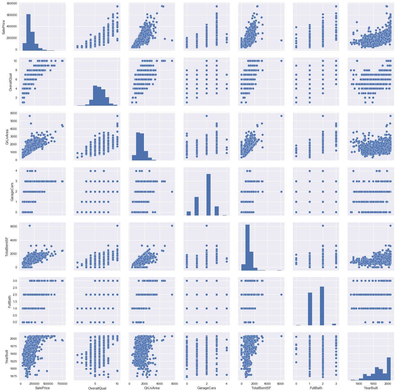
SalePrice 和相关变量之间的散点图
sns.set()
cols = ['SalePrice', 'OverallQual', 'GrLivArea','GarageCars', 'TotalBsmtSF', 'FullBath', 'YearBuilt']
sns.pairplot(train[cols], size = 2.5)
plt.show();
train[['SalePrice', 'OverallQual', 'GrLivArea','GarageCars', 'TotalBsmtSF', 'FullBath', 'YearBuilt']].info()
<class 'pandas.core.frame.DataFrame'>
RangeIndex: 1460 entries, 0 to 1459
Data columns (total 7 columns):
SalePrice      1460 non-null int64
OverallQual    1460 non-null int64
GrLivArea      1460 non-null int64
GarageCars     1460 non-null int64
TotalBsmtSF    1460 non-null int64
FullBath       1460 non-null int64
YearBuilt      1460 non-null int64
dtypes: int64(7)
memory usage: 79.9 KB
二. 特征工程
test['SalePrice'] = None
train_test = pd.concat((train, test)).reset_index(drop=True)
1. 缺失值分析
- 根据业务,常识,以及第二步的数据分析构造特征工程.
- 将特征转换为模型可以辨别的类型(如处理缺失值,处理文本进行等)
total= train_test.isnull().sum().sort_values(ascending=False)
percent = (train_test.isnull().sum()/train_test.isnull().count()).sort_values(ascending=False)
missing_data = pd.concat([total, percent], axis=1, keys=['Total','Lost Percent'])

print(missing_data[missing_data.isnull().values==False].sort_values('Total', axis=0, ascending=False).head(20))


'''
1. 对于缺失率过高的特征,例如 超过15% 我们应该删掉相关变量且假设该变量并不存在
2. GarageX 变量群的缺失数据量和概率都相同,可以选择一个就行,例如:GarageCars
3. 对于缺失数据在5%左右(缺失率低),可以直接删除/回归预测
'''
'\n1. 对于缺失率过高的特征,例如 超过15% 我们应该删掉相关变量且假设该变量并不存在\n2. GarageX 变量群的缺失数据量和概率都相同,可以选择一个就行,例如:GarageCars\n3. 对于缺失数据在5%左右(缺失率低),可以直接删除/回归预测\n'
train_test = train_test.drop((missing_data[missing_data['Total'] > 1]).index.drop('SalePrice') , axis=1)
# train_test = train_test.drop(train.loc[train['Electrical'].isnull()].index)

tmp = train_test[train_test['SalePrice'].isnull().values==False]
print(tmp.isnull().sum().max()) # justchecking that there's no missing data missing
1
2. 异常值处理
单因素分析
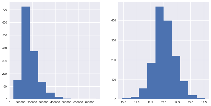
这里的关键在于如何建立阈值,定义一个观察值为异常值。我们对数据进行正态化,意味着把数据值转换成均值为 0,方差为 1 的数据
fig = plt.figure(figsize=(12, 6))
ax1 = fig.add_subplot(1, 2, 1)
ax2 = fig.add_subplot(1, 2, 2)
ax1.hist(train.SalePrice)
ax2.hist(np.log1p(train.SalePrice))

'''
从直方图中可以看出:

* 偏离正态分布
* 数据正偏
* 有峰值
'''
# 数据偏度和峰度度量:

print("Skewness: %f" % train['SalePrice'].skew())
print("Kurtosis: %f" % train['SalePrice'].kurt())

'''
低范围的值都比较相似并且在 0 附近分布。
高范围的值离 0 很远,并且七点几的值远在正常范围之外。
'''
'\n低范围的值都比较相似并且在 0 附近分布。\n高范围的值离 0 很远,并且七点几的值远在正常范围之外。\n'
双变量分析
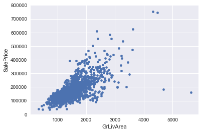
1.GrLivArea 和 SalePrice 双变量分析
var = 'GrLivArea'
data = pd.concat([train['SalePrice'], train[var]], axis=1)
data.plot.scatter(x=var, y='SalePrice', ylim=(0,800000));

'''
从图中可以看出:

1. 有两个离群的 GrLivArea 值很高的数据,我们可以推测出现这种情况的原因。
    或许他们代表了农业地区,也就解释了低价。 这两个点很明显不能代表典型样例,所以我们将它们定义为异常值并删除。
2. 图中顶部的两个点是七点几的观测值,他们虽然看起来像特殊情况,但是他们依然符合整体趋势,所以我们将其保留下来。
'''
'\n从图中可以看出:\n\n1. 有两个离群的 GrLivArea 值很高的数据,我们可以推测出现这种情况的原因。\n 或许他们代表了农业地区,也就解释了低价。 这两个点很明显不能代表典型样例,所以我们将它们定义为异常值并删除。\n2. 图中顶部的两个点是七点几的观测值,他们虽然看起来像特殊情况,但是他们依然符合整体趋势,所以我们将其保留下来。\n'
# 删除点
print(train.sort_values(by='GrLivArea', ascending = False)[:2])
tmp = train_test[train_test['SalePrice'].isnull().values==False]

train_test = train_test.drop(tmp[tmp['Id'] == 1299].index)
train_test = train_test.drop(tmp[tmp['Id'] == 524].index)
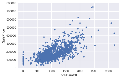
2.TotalBsmtSF 和 SalePrice 双变量分析
var = 'TotalBsmtSF'
data = pd.concat([train['SalePrice'],train[var]], axis=1)
data.plot.scatter(x=var, y='SalePrice',ylim=(0,800000))
核心部分
“房价” 到底是谁?
这个问题的答案,需要我们验证根据数据基础进行多元分析的假设。
我们已经进行了数据清洗,并且发现了 SalePrice 的很多信息,现在我们要更进一步理解 SalePrice 如何遵循统计假设,可以让我们应用多元技术。
应该测量 4 个假设量:
- 正态性
- 同方差性
- 线性
- 相关错误缺失
正态性:
应主要关注以下两点:直方图 – 峰度和偏度。
正态概率图 – 数据分布应紧密跟随代表正态分布的对角线。
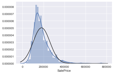
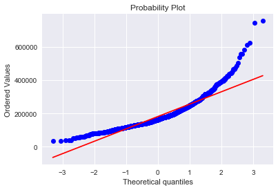
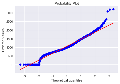
- SalePrice 绘制直方图和正态概率图:
sns.distplot(train['SalePrice'], fit=norm)
fig = plt.figure()
res = stats.probplot(train['SalePrice'], plot=plt)
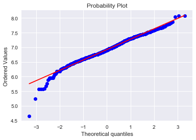
'''
可以看出,房价分布不是正态的,显示了峰值,正偏度,但是并不跟随对角线。
可以用对数变换来解决这个问题
'''
'\n可以看出,房价分布不是正态的,显示了峰值,正偏度,但是并不跟随对角线。\n可以用对数变换来解决这个问题\n'
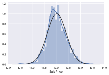
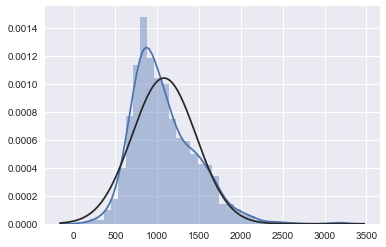
# 进行对数变换:
# 进行对数变换:
train_test['SalePrice'] = [i if i is None else np.log1p(i) for i in train_test['SalePrice']]
# 绘制变换后的直方图和正态概率图:
tmp = train_test[train_test['SalePrice'].isnull().values==False]

sns.distplot(tmp[tmp['SalePrice'] !=0]['SalePrice'], fit=norm);
fig = plt.figure()
res = stats.probplot(tmp['SalePrice'], plot=plt)
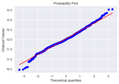
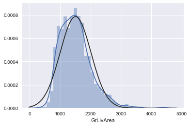
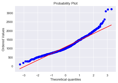
2. GrLivArea
绘制直方图和正态概率曲线图:
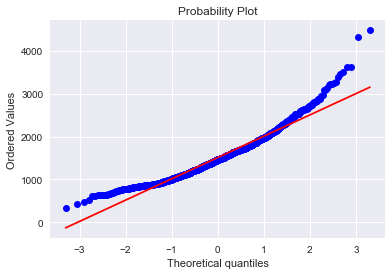
sns.distplot(train['GrLivArea'], fit=norm);
fig = plt.figure()
res = stats.probplot(train['GrLivArea'], plot=plt)
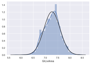
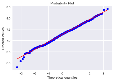
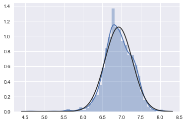
# 进行对数变换:
train_test['GrLivArea'] = [i if i is None else np.log1p(i) for i in train_test['GrLivArea']]

# 绘制变换后的直方图和正态概率图:
tmp = train_test[train_test['SalePrice'].isnull().values==False]
sns.distplot(tmp['GrLivArea'], fit=norm)
fig = plt.figure()
res = stats.probplot(tmp['GrLivArea'], plot=plt)
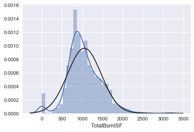
3.TotalBsmtSF
绘制直方图和正态概率曲线图:
sns.distplot(train['TotalBsmtSF'],fit=norm);
fig = plt.figure()
res = stats.probplot(train['TotalBsmtSF'],plot=plt)

'''
从图中可以看出:
* 显示出了偏度
* 大量为 0(Y值) 的观察值(没有地下室的房屋)
* 含 0(Y值) 的数据无法进行对数变换
'''
'\n从图中可以看出:\n* 显示出了偏度\n* 大量为 0(Y值) 的观察值(没有地下室的房屋)\n* 含 0(Y值) 的数据无法进行对数变换\n'
# 去掉为0的分布情况
tmp = train_test[train_test['SalePrice'].isnull().values==False]

tmp = np.array(tmp.loc[tmp['TotalBsmtSF']>0, ['TotalBsmtSF']])[:, 0]
sns.distplot(tmp, fit=norm)
fig = plt.figure()
res = stats.probplot(tmp, plot=plt)
# 我们建立了一个变量,可以得到有没有地下室的影响值(二值变量),我们选择忽略零值,只对非零值进行对数变换。
# 这样我们既可以变换数据,也不会损失有没有地下室的影响。

print(train.loc[train['TotalBsmtSF']==0, ['TotalBsmtSF']].count())
train.loc[train['TotalBsmtSF']==0,'TotalBsmtSF'] = 1
print(train.loc[train['TotalBsmtSF']==1, ['TotalBsmtSF']].count())
TotalBsmtSF    37
dtype: int64
TotalBsmtSF    37
dtype: int64
# 进行对数变换:
tmp = train_test[train_test['SalePrice'].isnull().values==False]

print(tmp['TotalBsmtSF'].head(10))
train_test['TotalBsmtSF']= np.log1p(train_test['TotalBsmtSF'])

tmp = train_test[train_test['SalePrice'].isnull().values==False]
print(tmp['TotalBsmtSF'].head(10))
0     856.0
1    1262.0
2     920.0
3     756.0
4    1145.0
5     796.0
6    1686.0
7    1107.0
8     952.0
9     991.0
Name: TotalBsmtSF, dtype: float64
0    6.753438
1    7.141245
2    6.825460
3    6.629363
4    7.044033
5    6.680855
6    7.430707
7    7.010312
8    6.859615
9    6.899723
Name: TotalBsmtSF, dtype: float64
# 绘制变换后的直方图和正态概率图:
tmp = train_test[train_test['SalePrice'].isnull().values==False]

tmp = np.array(tmp.loc[tmp['TotalBsmtSF']>0, ['TotalBsmtSF']])[:, 0]
sns.distplot(tmp, fit=norm)
fig = plt.figure()
res = stats.probplot(tmp, plot=plt)
同方差性:
最好的测量两个变量的同方差性的方法就是图像。
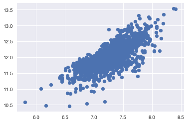
- SalePrice 和 GrLivArea 同方差性
绘制散点图:
tmp = train_test[train_test['SalePrice'].isnull().values==False]

plt.scatter(tmp['GrLivArea'], tmp['SalePrice'])
<matplotlib.collections.PathCollection at 0x11a366f60>
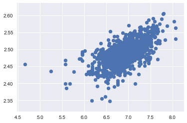
- SalePrice with TotalBsmtSF 同方差性
绘制散点图:
tmp = train_test[train_test['SalePrice'].isnull().values==False]

plt.scatter(tmp[tmp['TotalBsmtSF']>0]['TotalBsmtSF'], tmp[tmp['TotalBsmtSF']>0]['SalePrice'])

# 可以看出 SalePrice 在整个 TotalBsmtSF 变量范围内显示出了同等级别的变化。
<matplotlib.collections.PathCollection at 0x11d7d96d8>
三. 模型选择
1.数据标准化
tmp = train_test[train_test['SalePrice'].isnull().values==False]
tmp_1 = train_test[train_test['SalePrice'].isnull().values==True]

x_train = tmp[['OverallQual', 'GrLivArea','GarageCars', 'TotalBsmtSF', 'FullBath', 'YearBuilt']]
y_train = tmp[["SalePrice"]].values.ravel()
x_test = tmp_1[['OverallQual', 'GrLivArea','GarageCars', 'TotalBsmtSF', 'FullBath', 'YearBuilt']]

# 简单测试,用中位数来替代
# print(x_test.GarageCars.mean(), x_test.GarageCars.median(), x_test.TotalBsmtSF.mean(), x_test.TotalBsmtSF.median())

x_test["GarageCars"].fillna(x_test.GarageCars.median(), inplace=True)
x_test["TotalBsmtSF"].fillna(x_test.TotalBsmtSF.median(), inplace=True)
2.开始建模
- 可选单个模型模型有 线性回归(Ridge、Lasso)、树回归、GBDT、XGBoost、LightGBM 等.
- 也可以将多个模型组合起来,进行模型融合,比如voting,stacking等方法
- 好的特征决定模型上限,好的模型和参数可以无线逼近上限.
- 我测试了多种模型,模型结果最高的随机森林,最高有0.8.
bagging:
单个分类器的效果真的是很有限。 我们会倾向于把N多的分类器合在一起,做一个“综合分类器”以达到最好的效果。 我们从刚刚的试验中得知,Ridge(alpha=15)给了我们最好的结果。
from sklearn.linear_model import Ridge
from sklearn.model_selection import cross_val_score
from sklearn.ensemble import BaggingRegressor, RandomForestRegressor
ridge = Ridge(alpha=0.1)
# bagging 把很多小的分类器放在一起,每个train随机的一部分数据,然后把它们的最终结果综合起来(多数投票)
# bagging 算是一种算法框架
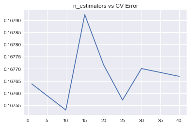
params = [1, 10, 20, 40, 60]
test_scores = []
for param in params:
clf = BaggingRegressor(base_estimator=ridge, n_estimators=param)
# cv=5表示cross_val_score采用的是k-fold cross validation的方法,重复5次交叉验证
# scoring='precision'、scoring='recall'、scoring='f1', scoring='neg_mean_squared_error' 方差值
test_score = np.sqrt(-cross_val_score(clf, x_train, y_train, cv=10, scoring='neg_mean_squared_error'))
test_scores.append(np.mean(test_score))
print(test_score.mean())
plt.plot(params, test_scores)
plt.title('n_estimators vs CV Error')
plt.show()
# 模型选择
## LASSO Regression :
lasso = make_pipeline(RobustScaler(), Lasso(alpha=0.0005, random_state=1))
* Elastic Net Regression
ENet = make_pipeline(
    RobustScaler(), ElasticNet(
        alpha=0.0005, l1_ratio=.9, random_state=3))
Kernel Ridge Regression
KRR = KernelRidge(alpha=0.6, kernel='polynomial', degree=2, coef0=2.5)
## Gradient Boosting Regression
GBoost = GradientBoostingRegressor(
    n_estimators=3000,
    learning_rate=0.05,
    max_depth=4,
    max_features='sqrt',
    min_samples_leaf=15,
    min_samples_split=10,
    loss='huber',
    random_state=5)
## XGboost
model_xgb = xgb.XGBRegressor(
    colsample_bytree=0.4603,
    gamma=0.0468,
    learning_rate=0.05,
    max_depth=3,
    min_child_weight=1.7817,
    n_estimators=2200,
    reg_alpha=0.4640,
    reg_lambda=0.8571,
    subsample=0.5213,
    silent=1,
    random_state=7,
    nthread=-1)
## lightGBM
model_lgb = lgb.LGBMRegressor(
    objective='regression',
    num_leaves=5,
    learning_rate=0.05,
    n_estimators=720,
    max_bin=55,
    bagging_fraction=0.8,
    bagging_freq=5,
    feature_fraction=0.2319,
    feature_fraction_seed=9,
    bagging_seed=9,
    min_data_in_leaf=6,
    min_sum_hessian_in_leaf=11)
## 对这些基本模型进行打分
score = rmsle_cv(lasso)
print("\nLasso score: {:.4f} ({:.4f})\n".format(score.mean(), score.std()))
score = rmsle_cv(ENet)
print("ElasticNet score: {:.4f} ({:.4f})\n".format(score.mean(), score.std()))
score = rmsle_cv(KRR)
print(
    "Kernel Ridge score: {:.4f} ({:.4f})\n".format(score.mean(), score.std()))
score = rmsle_cv(GBoost)
print("Gradient Boosting score: {:.4f} ({:.4f})\n".format(score.mean(),
                                                          score.std()))
score = rmsle_cv(model_xgb)
print("Xgboost score: {:.4f} ({:.4f})\n".format(score.mean(), score.std()))
score = rmsle_cv(model_lgb)
print("LGBM score: {:.4f} ({:.4f})\n".format(score.mean(), score.std()))
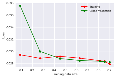
from sklearn.linear_model import Ridge
from sklearn.model_selection import learning_curve

ridge = Ridge(alpha=0.1)

train_sizes, train_loss, test_loss = learning_curve(ridge, x_train, y_train, cv=10,
                                                    scoring='neg_mean_squared_error',
                                                    train_sizes = [0.1, 0.3, 0.5, 0.7, 0.9 , 0.95, 1])

# 训练误差均值
train_loss_mean = -np.mean(train_loss, axis = 1)
# 测试误差均值
test_loss_mean = -np.mean(test_loss, axis = 1)

# 绘制误差曲线
plt.plot(train_sizes/len(x_train), train_loss_mean, 'o-', color = 'r', label = 'Training')
plt.plot(train_sizes/len(x_train), test_loss_mean, 'o-', color = 'g', label = 'Cross-Validation')

plt.xlabel('Training data size')
plt.ylabel('Loss')
plt.legend(loc = 'best')
plt.show()
mode_br = BaggingRegressor(base_estimator=ridge, n_estimators=10)
mode_br.fit(x_train, y_train)
y_test = np.expm1(mode_br.predict(x_test))
四 建立模型
模型融合 voting
# 模型融合
class AveragingModels(BaseEstimator, RegressorMixin, TransformerMixin):
    def __init__(self, models):
        self.models = models

    # we define clones of the original models to fit the data in
    def fit(self, X, y):
        self.models_ = [clone(x) for x in self.models]

        # Train cloned base models
        for model in self.models_:
            model.fit(X, y)

        return self

    # Now we do the predictions for cloned models and average them
    def predict(self, X):
        predictions = np.column_stack(
            [model.predict(X) for model in self.models_])
        return np.mean(predictions, axis=1)


# 评价这四个模型的好坏
averaged_models = AveragingModels(models=(ENet, GBoost, KRR, lasso))
score = rmsle_cv(averaged_models)
print(" Averaged base models score: {:.4f} ({:.4f})\n".format(score.mean(),
                                                              score.std()))

# 最终对模型的训练和预测
# StackedRegressor
stacked_averaged_models.fit(train.values, y_train)
stacked_train_pred = stacked_averaged_models.predict(train.values)
stacked_pred = np.expm1(stacked_averaged_models.predict(test.values))
print(rmsle(y_train, stacked_train_pred))

# XGBoost
model_xgb.fit(train, y_train)
xgb_train_pred = model_xgb.predict(train)
xgb_pred = np.expm1(model_xgb.predict(test))
print(rmsle(y_train, xgb_train_pred))
# lightGBM
model_lgb.fit(train, y_train)
lgb_train_pred = model_lgb.predict(train)
lgb_pred = np.expm1(model_lgb.predict(test.values))
print(rmsle(y_train, lgb_train_pred))
'''RMSE on the entire Train data when averaging'''

print('RMSLE score on train data:')
print(rmsle(y_train, stacked_train_pred * 0.70 + xgb_train_pred * 0.15 +
            lgb_train_pred * 0.15))
# 模型融合的预测效果
ensemble = stacked_pred * 0.70 + xgb_pred * 0.15 + lgb_pred * 0.15
# 保存结果
result = pd.DataFrame()
result['Id'] = test_ID
result['SalePrice'] = ensemble
# index=False 是用来除去行编号
result.to_csv('/Users/liudong/Desktop/house_price/result.csv', index=False)
